Reader on GPS positioning

This reader gives an introduction to Global Positioning Systems. A static version of this document is available in pdf.

Introduction

The NAVigation Satellite Time And Ranging (NAVSTAR) system, better known as the Global Positioning System (GPS), is one the most successful satellite systems to date. GPS is a one way radio ranging system which provides real-time knowledge of one's own position and a very accurate time reference. GPS is said to provide Positioning, Navigation and Timing (PNT) functionality, which is very valuable not only for the US military, for which it was first developed, but also to a myriad of commercial activities as well as the general public at large.

The GPS system consists of 3 segments:

The space segment, consisting of 24, or more satellites, with accurate atomic clocks on board, continuously transmits ranging signals to the Earth.
The control segment, consisting of a number of ground stations, which monitors the satellites, computes their orbits and clock offsets, and uploads this information to the satellites, which in turn encode this information on the ranging signal.
The user segment, simply consisting of a GPS receiver, which tracks 4 or more GPS satellites, and computes its own position.

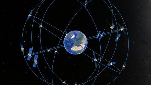
Fig. 1: GPS constellation with 24-32 satellites in 6 orbital planes (figure created with Google Earth™; satellite model from grabcad).

The success of GPS is strongly linked to the ever decreasing costs of GPS receivers. Although high-end receivers still cost in the order of $10k, mass-market receivers, such as those used in smart-phones, cost no more than a few dollars each. In 2015 there were an estimated 3.6 billion GPS-capable devices (ESA, 2015), the vast majority of which are smart-phones.

Ranging

The GPS satellites transmit signals in the L band (i.e. 1 to 2 GHz range) of the radio frequency spectrum. GPS uses Code Division Multiple Access (CDMA) to allow different satellites to send signals at exactly the same center frequency without interfering with each other. The signal consists of a carrier wave on which each satellite modulates its own unique Pseudo Random Noise (PRN) spreading code (see fig. 2) and, at a low-rate, the satellite orbit and clock information. The signals arrives at the receiver with a unknown delay, and due to the relative velocity of the GPS satellites with respect to a GPS user, with an unknown Doppler frequency shift.

A GPS receiver typically consists of tens of so-called channels, and will allocate each of these to a specific GPS satellite. When a GPS receiver first starts up, it will begin to search for a particular GPS satellite on each of its channels, by scanning (trying) for the corresponding spreading codes at different Doppler offsets and time delays. This is done by overlaying the received signal with a local copy of the same code and then (time) shifting it until correlation shows a maximum (best fit, or match). Once the receiver has locked onto the spreading code, it can start taking pseudorange code and Doppler frequency measurements, which are basically the shift in time and the shift in frequency that are required to maintain the tracking lock (onto the received satellite signal). Through the pseudorange, the receiver measures the travel-time of the radio signal from satellite to receiver: τ_r^s = t_r - t^s, where t^s is the time the signal was transmitted by the satellite, and t_r is the time the signal was received at the receiver, noting that these clocks may, to some extent, deviate from the true time. The measured travel-time is converted into the pseudorange through p_r^s = cτ_r^s, by multiplying by the speed of light c.

The pseudorange represents the travel time of the signal, and is also affected by the (known) satellite clock offset, the (unknown) receiver clock offset, and a number of additional delays (treated below), all multiplied by the speed of light.

Fig. 2: GPS L1C/A signal is composed of a carrier wave (sinusoid, not to scale), a spreading code (a sequence of 0 and 1 bits/chips), and a low-rate navigation data message. Both the spreading code and navigation message are phase-modulated on the carrier wave, through a technique called Binary Phase Shift Keying (BPSK). For the CA-code, the spreading codes are all publicly available, and GPS-receivers have them built-in.

Additionally, the receiver may measure the (fractional) phase-difference between the received carrier from the satellite and a locally generated copy. And, it can keep track of the number of cycles of the carrier wave since the start of tracking, together known as the carrier phase measurement. The carrier wave measurement is a very precise measure of the distance between the satellite and the receiver, but the initial number of cycles is unknown, and needs to be estimated before the carrier phase measurements can be used. The much better precision of the carrier phase measurement with respect to the pseudorange code measurement can be understood form fig. 2, since the carrier wavelength is much smaller than the code chip length (1575 wavelengths of the carrier fit in one chip of the Pseudo Random Noise (PRN) spreading code). Finally, the receiver can also measure the signal-to-noise ratio (SNR, based on the received signal-strength), which gives an indication of the quality of the measurement.

Multi-frequency

One of the main error sources in GPS is due to the ionosphere, which delays the signals, and thus affects the range measurements. One way of dealing with this is to track signals from the same satellite on two or more frequencies. The ionosphere delay scales with the inverse of the radio frequency squared, and this relation can be used to create the so-called ionosphere-free range measurements. For this reason the GPS satellites were originally designed to transmit ranging signals on both the L1 (1575.42 MHz) and L2 (1227.60 MHz) frequency.

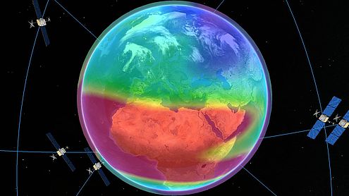
Fig. 3: The Earth's ionosphere delays GPS signals. The largest delays occur round the geomagnetic equator around local noon, and during solar maxima. The ionospheric delay may be highly variable, as a function of both time and space (figure created with Google Earth™; ionosphere layer from ES4D; satellite model from grabcad).

Positioning

GPS positioning is based on the concept of lateration (not triangulation). By measuring the distance to a number of GPS satellites, and using the known satellite positions, the GPS receiver can compute its own position. To estimate the three position coordinates and the receiver time offset, a GPS receiver needs to track at least 4 satellites. The reason one satellite is also needed to accurately compute the time is illustrated in fig. 4, for a 2-dimensional example. In this figure, the black dots indicate the known satellite positions. If the range to one satellite is known, we can draw a circle around the satellite position, on which the receiver must be located. If the range to a second satellite is known, we can draw another circle and the intersections of the two circles are the possible receiver position.

However, in GPS positioning we do not actually have ranges, but rather pseudoranges, which still include the unknown receiver clock offset. The receiver clock offset equally impacts the measurements to all satellites, reflected by the radii of the coloured circles in fig. 4. Since we do not yet know the receiver clock offset, we do not know whether we should consider the green, blue, purple, or magenta circles. Note that any of the two circles intersect each other for different time offsets (different colours). That means that if the time is not known accurately, neither is the position. However, three circles only intersect each other at a single point for one time offset (the blue circles). That shows that the time offset can be determined as well as the position. If the receiver time offset is already known, e.g. because it is connected to an atomic clock, one fewer satellite would be required.

Fig. 4: GPS works on the basis of lateration; here is a 2-dimensional example. If the distances to enough satellites are known (measured), the receiver position can be determined by intersecting circles around the satellites with radii equal to the measured distances. In GPS processing, the receiver clock offset is also unknown, which means one additional satellite is required to solve the problem. In 3-dimensions, measurements to at least 4 satellites are needed to determine the 3-dimensional user position, and the receiver clock offset.

Pseudorange observation equation

The pseudorange measurement can be written as:

p_r^s = √(xs-x_r)2+(ys-y_r)2+(zs-z_r)2 + b + ε

in which xs, ys and zs are the satellite coordinates at the time of signal transmission, x_r, y_r and z_r are the receiver coordinates at time of signal reception, b contains the receiver clock offset and systematic delays (times the speed of light c) and ε is the random measurement noise. Note that, if the receiver clock is ahead of GPS system time, b is positive, and the measured pseudoranges are 'too long'.

In practice, as one typically observes more satellites than the minimum of four, GPS positioning does not actually involve drawing circles or spheres, but works on the principle of least squares estimation. First the observation model is defined, which links the observations to the unknown parameters in a matrix equation. Since the GPS model is non-linear, the step involves a linearisation around an approximate position. A least squares algorithm is then used to solve this matrix equation, which can contain more observations than unknown parameters; while minimizing the uncertainty of the solution (see the Primer on Mathematical Geodesy, chapter 4). Similar to the position coordinate computation from the pseudorange measurements, the 3D velocity vector of the receiver can be computed from the Doppler-shift measurements.

Reference systems

GPS yields Cartesian coordinates (x,y,z) in WGS84, a realization of the World Geodetic System. These can be transformed into latitude (φ), longitude (λ), and ellipsoidal height (h). In differential mode (introduced below), the computed coordinates are in the same reference system as the base station coordinates, which are generally provided in a local or regional reference system (e.g. ETRS89 in Europe, a realization of the European Terrestrial Reference System). More information about these different reference systems and transformations from one to another can be found in the reader on Reference Systems for Surveying and Mapping.

GPS accuracy

The quality of the GPS position solution is largely dependent on the number of available satellites and their geometry with respect to the user. If enough satellites are visible on all sides of the receiver (e.g. fig. 5), a good position accuracy can be expected. In this case the only weakness in the geometry is the fact that there are no satellites beneath the receiver, which is generally the case, as one cannot track and observe satellites below the horizon. As a result vertical accuracy is generally poorer than the horizontal accuracy by about a factor of 1.5.

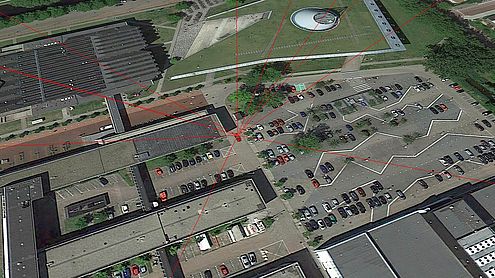
Fig. 5: Satellite to receiver line-of-sight for all GPS satellites above the horizon at the TU Delft library parking (figure created with Google Earth™; vehicle model from carssiv).

In many situations one or more satellite signals are blocked by surrounding buildings or other obstacles which is called shadowing see fig. 6. In this case GPS performance might be significantly degraded. Furthermore, in built-up areas, GPS receivers often experience signal reflections, i.e. signals arrive at the receiver after bouncing off an object (multipath). Since the reflected signal path is always longer than the direct path, this causes an error in the range measurement (see the purple line in fig. 6). It is also possible that both the direct and reflected signals arrive at the receiver. In this case, the receiver must deal with the superposition of these signals, generally resulting in a biased range measurement.

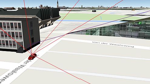
Fig. 6: Buildings and other objects may block the line-of-sight signal (shadowing), and/or cause signal reflections known as multipath (figure created with Google Earth™; vehicle model from carssiv).

The accuracy of standalone positioning with GPS, in the order of 5-15 meters under reasonable satellite visibility, is limited by the accuracy of the range measurements. The GPS measurements contain errors due to inaccurate satellite orbit and clock information, delays along the path of the signal, including atmosphere delays (ionosphere and troposphere), local effects including multipath, and measurement noise (see fig. 7).

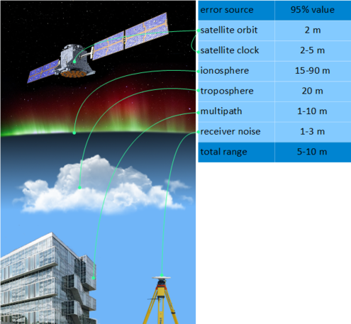
Fig. 7: Contributions to the GPS measurement errors. NOTE: Errors are in the range domain after Klobuchar ionosphere model corrections (about 50% reduction), and a-priori troposphere corrections (about 90% reduction); values based on experience. Image source: ESA 1 2; clipartpng; Aronsohn; Trimble.

GPS positioning modes

Several techniques have been developed to improve on the GPS Standard Positioning Service (SPS) accuracy. Firstly, GPS satellites generate a second, more precise, code on the same carrier wave, to provide the Precise Positioning Service (PPS). However, this code is encrypted and can only be used by the US military. Fortunately, even more accurate positioning modes are available.

Differential GPS (DGPS) uses a data link to a local base station, i.e. another GPS receiver at an accurately known position, and the relative position between the two is obtained. Measurement data from this base station are used, to reduce the effects of the atmospheric delays, satellite clock offsets and orbit errors. This can be achieved by differencing the observations from both receivers to the same satellites, which eliminates these (common) errors, which affect both receivers almost identically if the distance between them is small enough (5-10km). From the differenced observations, the baseline (vector) between the two receivers can be computed through least squares estimation. The position of the rover is then obtained by adding the baseline to the accurately known coordinates of the reference station (see fig. 8).

Fig. 8: Differential GPS combines data from a roving receiver with data from a (reference) base station; the position of the rover is actually computed relative to the base station. A number of errors, including the atmospheric errors, is almost identical for two receivers in close proximity to each other. Hence, these errors cancel in relative positioning. Image source: USAF; dreamstime.

To obtain the highest possible accuracy from GPS it is no longer sufficient to use only the pseudorange code measurements, rather the previously introduced carrier phase measurements are required. As mentioned before, this does pose the problem of the unknown initial number of cycles, also called the carrier wave ambiguity, which need to be estimated together with the other unknown parameters.

An ambiguity consists of a fractional part at the satellite (equal for both receivers, and already removed by the differencing between the base station and rover), a fractional part at the receiver (equal for all tracked satellites), and an integer number of whole cycles. This fact is exploited in a technique called Real-Time Kinematic (RTK), or carrier-phase baseline processing if performed in post processing, by selecting a reference satellite and forming a second difference between the measurement to the reference satellite and all other satellites, to eliminate the fractional part at the side of the receiver. In this special case the (double-differenced) carrier phase ambiguities can be resolved to their integer number very efficiently through integer least-squares estimation. After only a few minutes, cm position accuracy can be realized. The requirement for a nearby reference receiver is a disadvantage of RTK considering effort and/or cost.

Fig. 9: Excavator in the process of constructing a motorway embankment, as an example of machine guidance. GPS-RTK provides accurate real-time position information (note the two GPS-antennas on the back of the engine). Image courtesy of Heijmans.

Many high-end GPS receivers have RTK functionality built in, but it can also be performed with professional software, or even with the open source RTKLIB program package.

In those instances where a nearby reference receiver (or network) is not available or cost-prohibitive, Precise Point Positioning (PPP) is an attractive alternative. PPP only relies on a global, very sparse network of reference receivers (e.g. some 40 receivers worldwide), which monitor the GPS satellites and compute corrections to the errors in the satellite orbits and clocks. Conventional PPP uses dual frequency data to eliminate the ionosphere delay, while a low-cost variant uses single frequency data with a (predicted) ionosphere model. The fractional carrier phase ambiguities cannot be eliminated, which means that integer least-squares estimation is not possible. Ambiguities can still be estimated as constant values though, since an ambiguity does not change as long as the receiver keeps tracking the satellite, a fact used in the PPP data processing.

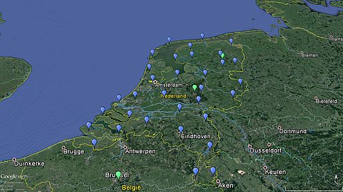
Fig. 10: Example of a dense local GPS reference network used for RTK in the Netherlands in blue, and a sparse global network used for PPP in green (figure created with Google Earth™).

However, because the ambiguities cannot be fixed to integer values, PPP suffers from a longer convergence period than RTK. After a convergence period in which the accuracy of the estimated ambiguities improves gradually, the PPP solution starts relying more and more on the phase measurements. The eventual position accuracy for dual frequency PPP can reach cm, or even mm level, while single frequency PPP can reach an accuracy of a few dm.

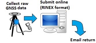
Fig. 11: Natural Resources Canada offers a free on-line PPP service for post processing. To obtain a PPP solution, submit previously recorded data to the NRCan website (after login). Image source: NRCan.

Much research effort is spent to try and combine the best aspects of PPP and RTK, i.e. using a sparse (global) reference network and ambiguity resolution. Wide Area RTK and PPP-RTK are based on the principles of RTK, but try to stretch the inter-station distances to several hundreds of km, while PPP AR starts from the global PPP network, and tries to solve the problem of ambiguity resolution. The ultimate goal is to achieve high-precision positioning across a (very) large area.

Another development is to bring high-accuracy positioning techniques, e.g. RTK and PPP, to low-cost devices. An example is that of the RTK kits that can be ordered from u-blox or emlid. Another example is the porting of the RTKLIB software to the android platform (see fig. 12). The RTKGPS+ app can combine measurements from a GPS receiver, connected to the smart phone via USB, with corrections retrieved through the internet connection of the phone to compute an accurate position.

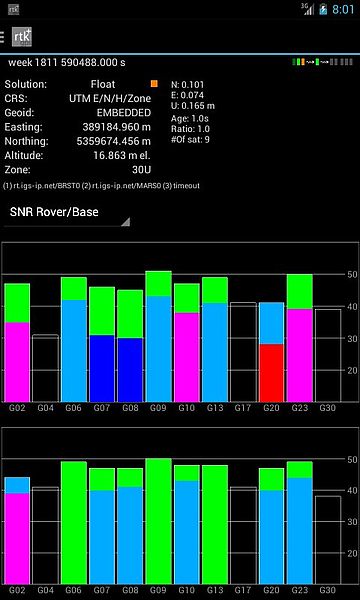
Fig. 12: RTKGPS+, an Android port of the RTKLIB software, brings high-accuracy positioning techniques to the smart phone. Note: the software relies on an external GPS device to obtain the pseudorange and carrier phase measurements. Image source: appstore.

Satellite Based Augmentation Systems (SBAS), e.g. the European EGNOS system, designed to enable GPS-based aeroplane precision approaches, rely on the same principals as PPP. However, given the primary application, the focus is on integrity not accuracy; carrier phase measurements are only used to smooth the pseudorange solution. An additional advantage of using SBAS is that the corrections are transmitted on the same frequency as GPS itself, so no additional data link is necessary.

Processing strategies, dynamic model and observation period

As already hinted at, the GPS position accuracy improves when the measurement time duration increases. One important factor here is the dynamic model, or how the measurement epochs can be linked to each other. If the receiver is stationary, the improvement will be most notable, as we can basically estimate a single position from many measurements. The position accuracy of a static receiver is shown as a function of the measurement duration in fig. 13 for each of the previously treated GPS processing strategies.

For a moving receiver the accuracy can also improve over time, if some of the other parameters can be kept constant, e.g. the ambiguities, or if the movement can be constrained or predicted to some extent based on the current position (e.g. a car driving on a straight line, at constant velocity). This can be implemented with a Kalman filter or a recursive least squares data processing algorithm.

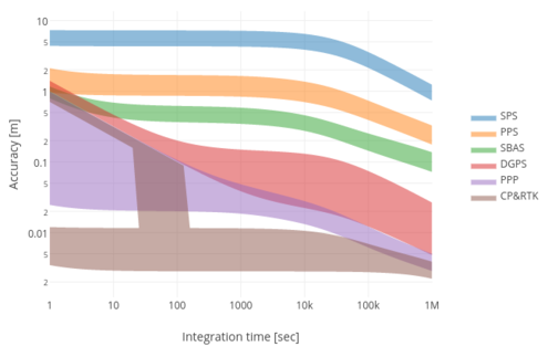
Fig. 13: Accuracies of various GPS positioning modes for a static receiver (courtesy of Hans van der Marel). The integration time is the total measurement duration, along the horizontal axis, and the position coordinates accuracy is along the vertical axis. Note the logarithmic scales.

Two related issues are:

The difference between real-time processing, and post-processing (after the fact), where post-processed results are generally more accurate, but obviously not suitable for certain applications.
The measurement rate of the receiver. GPS receivers often take pseudorange code, carrier phase, Doppler and SNR measurements once every second, hence at 1 Hz, but depending on the application, 10-20 Hz is also common practice, and technically up to 100 Hz measurement rate is possible. To reduce the computational burden, data storage, and power requirement, lower measurement rates (e.g. once per 30s) are also common. The impact of the measurement rate on the position accuracy in marginal (a higher data rate can slightly improve precision), because the measurement errors are generally correlated in time. This means that measurements taken in quick succession are not independent.

Other Global Navigation Satellite Systems

Not to be dependent on a US military system, other countries have developed their own Global Navigation Satellite Systems (GNSS).

Presently, a significant increase in the available Global Navigation Satellite Systems, frequencies and signals is ongoing. GPS is in the process of modernization. This is achieved by following up older satellites by new satellites with expanded and improved capabilities. The civil L2C signal, for improved dual frequency performance, has becoming available on more and more satellites. Even more importantly, new GPS satellites also transmit an additional (wide-band) signal on the L5 frequency primarily designed for safety-of-life applications (higher chip-rate, hence shorter chip-length, and more accurate ranges).

The Russian GLObal NAvigation Satellite System (GLONASS), has been fully replenished and at present has 24 active satellites. Planned modernizations of GLONASS include an additional signal transmitted on the L5 frequency, and a switch from Frequency-Division Multiple Access (FDMA) to CDMA which would increase potential interoperability with other GNSS.

Galileo, the European GNSS, is still under development. The full Galileo constellation is planned to exist of 30 satellites by the end of 2020. The Galileo system will transmit navigation signals on four different carrier frequencies: L1/E1, L5/E5a, E5b and E6, two of which (E5a and E5b) can also be tracked together as one extra wide-band (Alt-BOC) signal with unprecedented accuracy.

The Chinese BeiDou Navigation Satellite System (BDS), sometimes still known as Compass, was designed to provide independent regional navigation in the first stage and global coverage by 2020. Currently the regional system is fully operational, and the first satellite of the second stage has already been launched starting the transition towards a global navigation system.

The realized and expected upgrades of and additions to the available GNSS signals can have a range of improvements on many GNSS applications. Some of the more important ones are: the higher ranging accuracy of the new signals, the availability of many more satellites at once (more satellites available to combat urban environments), and both the availability of more frequencies and satellites.

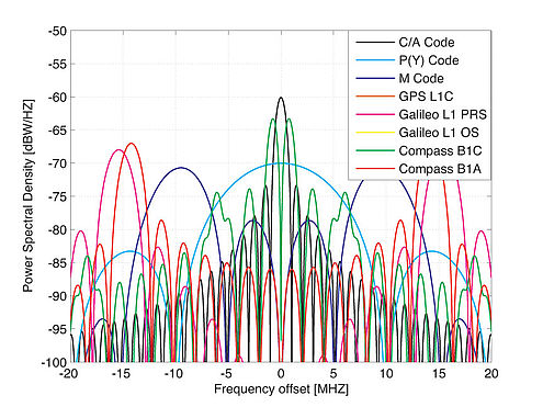
Fig. 14: The frequency spectrum in the L1 band has become quite crowded with the introduction of new systems and signals (the center of the graph corresponds to a frequency of 1575.42 MHz). Also considering that for each system, multiple satellites share the same frequency, extensive interoperability studies are performed to make sure the systems do not interfere with each other (figure from GPS World, 2010).

Multi-GNSS positioning also brings new challenges, as so-called Inter-System Biases (ISB) are introduced in the model. The system time as maintained by GPS may (will) not be the same as the system time as maintained for Galileo, for instance. Hence one has to account for the fact that these systems may have an offset in time with respect to each other. To use multiple systems simultaneously in an optimal manner, these biases must be studied, and if possible corrected or eliminated.

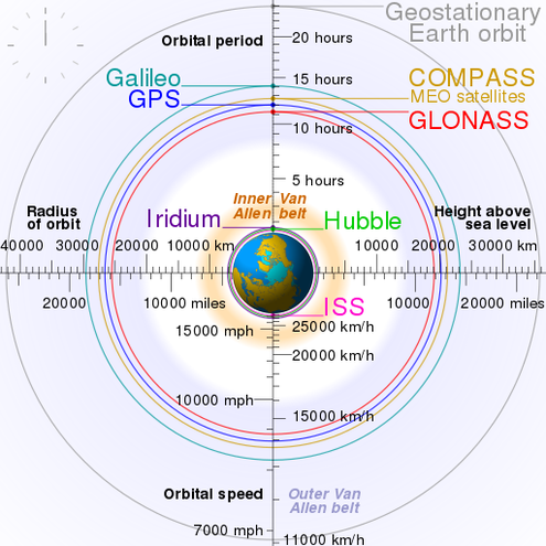
Fig. 15: Orbits of several navigation satellite systems. Most navigation satellites are in Medium Earth Orbits (MEO) with a radii between 25 and 30 thousand km. Several systems including the Chinese BeiDou system and the Satellite Based Augmentation Systems use satellites in geostationary orbits (figure from Wikimedia Commons).

Applications

There are many different applications of GPS positioning each with its own requirements and, related to that, a preferred processing strategy.

Smart-phones, car navigation, and personal navigation usually have the lowest requirements, and the GPS standard positioning service suffices.
Lane specific navigation advice for road users requires sub meter accuracy, which can be fulfilled with single frequency PPP.
Surveying for maps or construction, requires cm to mm and will use RTK if available, or PPP otherwise.
Deformation monitoring, due to earth quakes, volcanic activity, mining or extraction of petroleum or natural gas, as well as any number of scientific applications require the highest possible accuracy and use carrier phase baseline processing.
Aeroplane precision landing requires high integrity positioning, and can use SBAS to obtain this.
Machine guidance and self-driving vehicles require high-accuracy and integrity, this can be achieved by using GPS-RTK (possibly fused with additional sensors).

There is also a number of GPS applications, where the position computation is not the (primary) goal.

The accurate time (nano seconds), which the receiver computes as a by-product, is used in timing applications. GPS is used for timing in communication systems, electrical power grids, and financial networks.
Nuisance parameters such as the atmosphere delays can also be used as observations e.g. to model the ionosphere, or derive weather models from troposphere delays.
The GPS signals can also be used outside of their intended purpose, e.g. to determine sea-level height by measuring reflected GPS signals from orbit.

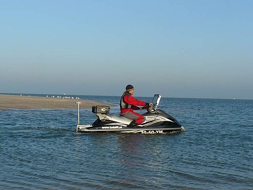
Fig. 16: A water scooter, equipped with an echo-sounder is used to monitor the sand engine (zandmotor), near the Dutch coast. High-precision GPS - note the antenna at the back of the water scooter - is used for positioning, in order to turn the echo-sounder depth-measurements into a sea-floor-map. Image courtesy of Matthieu de Schipper.

An extensive textbook, covering nearly any aspect of Global Navigation Satellite Systems, is the Springer Handbook of Global Navigation Satellite Systems, editors P.J.G. Teunissen and O. Montenbruck, 2017, DOI 10.1007/978-3-319-42928-1, ISBN 9783319429267 (print), ISBN 9783319429281 (online). This book, with 41 chapters on 1328 pages, is available as e-book through the TU Delft library.

Exercises

Question 1 What are the largest remaining error sources in short-baseline DGPS, explain your answer.

Answer 1 The atmosphere delays as well as the satellite orbit and clock errors are eliminated in DGPS, which leaves multipath and (pseudorange) measurement noise as the largest error sources (see fig. 7).

Question 2 If a certain application requires decimeter positioning accuracy, which GPS positioning modes can be considered? And for how long a time would we need to take measurements?

Answer 2 RTK provides decimeter or even centimeter accuracy as soon as the ambiguities can be fixed, which generally is (well) within 100 seconds, and even faster in post-processing. PPP can also provide decimeter accuracy after several minutes. DGPS can reach decimeter accuracy as well, but may take over an hour to do so. SBAS and standalone GPS often do not reach decimeter accuracy even after one or several days, especially in the vertical component (see fig. 13).

Peter F. de Bakker - Jan 2017