Comparing computers
Quantum computers and classical computers are made of the same building blocks—but the ways they behave couldn’t be more different.
A quantum computer is made out of the same building blocks as everyday computers – which scientists refer to as classical computers – the main difference being that the quantum counterparts obey the laws of the smallest particles: quantum mechanics. The laws of quantum mechanics allow these building blocks to exist in superposition – in multiple states at once.
In both classical computers and quantum computers information (stored on either classical bits or quantum qubits) is manipulated by performing logical operations. When the computation is completed, we need to retrieve the answer, which for quantum computers is done by measuring the qubits. An additional property quantum computers can exploit is the surprising phenomenon of entanglement.
One qubit can store the value of two numbers, and with each qubit that we add, we can store the value of twice as many possibilities.
Bits and Qubits
As we have the alphabet as a basis for communication in English – all words can be built out of these 26 letters – computers also have an ‘alphabet’: bits. Rather than 26 letters, bits can take two values: “0” or “1”. Just as letters are combined in books to form nice stories, your PC or smartphone combines millions of “0”s and “1”s for performing calculations, displaying a movie or loading your favorite cat gifs!
In quantum computers, the fundamental units of information are represented by quantum bits (qubits) – the quantum counterpart of the classical bit. Besides being exactly 0 or 1, a quantum bit can also be in any combination of 0 and 1, called a superposition.
Superposition
Superposition refers to the phenomenon that quantum objects can be multiple things at once. For our qubits, this means they can be any arbitrary combination of “0” and “1”, such as 40% “0” and 60% “1”. Although we do not experience superposition in our daily lives, it is a regular phenomenon on the quantum level. To get a feeling of what superposition means, imagine spinning a coin on its side on a table. Before it collapses to the table, you are uncertain of whether it is head or tails, and you may take it as being both. Similarly, a qubit can be both “0” and “1”.
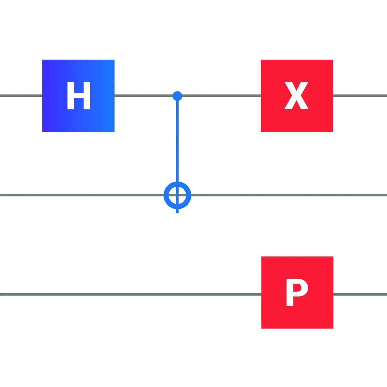
Logic Gates
In order to get anything meaningful out of our (qu)bits, we need to manipulate them. Say we have two numbers, 16 and 312, and we wish to multiply them. In a classical computer, we can convert these numbers into bits (see encoding information) and manipulate them, such that we get the correct answer. This is done using operations which are called logic gates – a sequence of actions which in our case represent multiplication. The result of this manipulation is passed on to new bits, which we can read out to get the result (which is 4992 if you’re curious).
Likewise, we need to manipulate our qubits in order to get anything meaningful out of the quantum computer. The major difference is that quantum logic gates do not compare bits and pass on the result to new bits – they manipulate the qubits directly. This means that as our quantum computer is running, it is constantly changing in which superposition of “0” and “1” each qubit is
Encoding Information
There are many ways of going from our human alphabet to the binary alphabet of computers. One such way is using the ASCII table, which is like a dictionary that translates “words” of eight bits (one byte) to our alphabet. For example, if we’d like to write DELFT, we’d need a total of 5x8=40 bits.
| D - 01000100 | E - 01000101 | L - 01001100 | F - 01000110 | T - 01010100 |
Quantum computing is more efficient with its qubits. Instead of using 40 qubits, we can encode “DELFT” in just 8 qubits by using a superposition of the ASCII codes of the five letters in this word. The downside is that we cannot readily get the entire word at once from this superposition – measurement will prevent us from obtaining “DELFT” in one go (see Measurement). Instead, when we measure these qubits, we will randomly get any of the letters in “DELFT”, each with a 20% probability.
Measurement
When the calculations are done, we’d like to know the results. For quantum computers, this is done by measuring the final data encoded in the qubits. However, what will you get when you measure something that can be 40% “0” and 60% “1”? The laws of quantum mechanics dictate that you will always measure either “0” or “1”, in our case with 40% and 60% probability – just like when you slap a spinning coin flat on the table, you will sometimes end up with heads and sometimes with tails. This means that when you run the exact same procedure twice, you may get different outcomes.
That is why quantum programmers need to be very careful to end with 100% “0” or 100% “1” when designing their algorithms. This means that when quantum computers explore many different possibilities in parallel, algorithms need to be cleverly designed so that they do not end up with just as many different solutions, each with a very small probability. They do so by minimizing the chances that you get the incorrect solutions, and amplifying the chance of the correct outcomes.
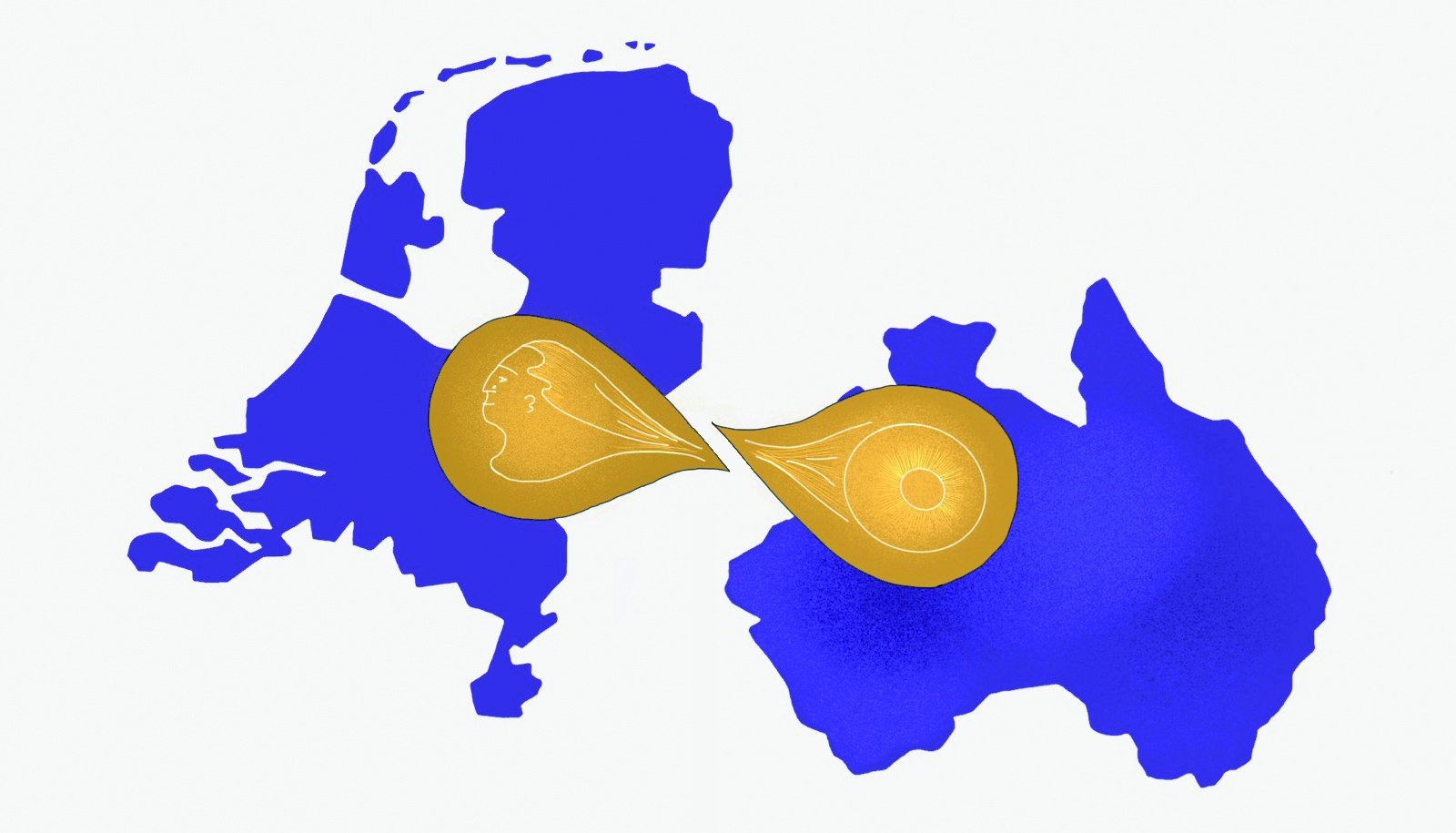
Entanglement
Qubits have another property which knows no classical analogue: entanglement. This property is that they can be correlated in a surprisingly tight way, even over long distances. Imagine you have two coins spinning on a table, and you measure them by smashing them one after the other. The probability that the first coin gives heads is 50%, and then when the first coin indeed came out as heads, the probability that the second coin gives heads is still 50%. If these coins were entangled, like we can do with qubits, this can change. We can entangle them such that if one coin ends up heads, then the other coin always gives heads too (and the same holds for tails).
The surprising property of entanglement is that this correlation persists over long distances. Let’s say I send you to Australia with one spinning coin of our entangled pair, and I remain in Delft with the other one. When you slap your spinning coin in Australia, and you find tails, you will immediately know what the outcome is when I slap my spinning coin in Delft – it will be tails too! This is something we do not experience at all in our daily lives – Einstein even referred to it as “spooky action at a distance”.
Exponential Power
It is common to see claims that quantum computers offer “exponential speedup” to computation or that they are “exponentially fast”. But what does this mean? In essence, quantum computers are not a kind of magical machine that will make all our devices faster. On the contrary: although quantum computers can be faster, this depends on the design of very specialized algorithms that can solve certain problems (see also Applications).
So what is this “exponential speedup”? Quantum computing is efficient with the information it can process through its qubits. It needs less qubits to encode the word “DELFT” than classical computers need bits. And this efficiency grows immensely when the number of qubits increases. One qubit can store the value of two numbers, and with each qubit that we add to our computer, we can store the value of twice as many possibilities. This exponential growth means that a 50-qubit quantum computer can capture a thousand million million numbers –more than there are stars in the Milky Way. Imagine what amount of information we can process with a 100- or even 1000-qubit quantum computer.